GenBench: real-world genomics benchmarks for R
Bioinformatics is growing as a market and as a field. Just looking at the diversity of questions covered by Bioconductor shows us that "bioinformatics" is no longer just the realm of sequence comparison.
BeDataDriven, the Dutch company behind Renjin, has recently become involved in bioinformatics, and needed a base of representative testing/benchmarking code to help develop Renjin for bioinformatics applications.
Background
Forked from and inspired by GenBase, GenBench is an attempt to build up some ecologically valid benchmarks and tests for bioinformatics. Another nice example of this is RforProteomics, see their project and accompanying paper.
This benchmark does not cover all possible operations performed in bioinformatics/genomics. In particular, we chose to not focus on (pre-)processing of raw data and instead focus on higher-level processing typical for a range of datatypes. We have examples for microarray and mRNA-seq, some proteomics and genetics, machine learning and data integration (for full information, also on the data sources, see the end of the post).
We also chose to use real-world data, to allow not just benchmarking of clock speeds upon completion of a given analysis, but also to allow for testing.
Generally speaking, we do not endorse any of the methods used as "standards" or "recommended", in fact, because we aim to start simple and avoid as far as possible non-essential packages, methods may be very much not recommended. Future updates will implement more advanced methods, a wider range of packages, etc.
Suggestions and contributions for datasets or methods are welcome.
This post
In this post we wanted to get feedback on "version 1.0" of GenBench, and thought a nice way to do that would be to run a little experiment in the hope it would generate interest/support/glory.
Currently (as of June 2015) GenBench includes ten benchmark scripts, each containing several microbenchmarks, covering topics from microarray analysis with limma, graphs with iGraph and some machine learning as might be applied to patient profiling. We thought this was enough to make some comparisons across different versions of R, to examine the real-world effects of recent upgrades to GNU R.
Specifically, we ran the full suite of benchmarks against the following releases (compiled from source using this script:
- R-2.14.2
- R-2.15.3
- R-3.0.3
- R-3.1.3
- R-3.2.0
Running the benchmarks
After installing the various versions of GNU R, we set up a Jenkins build job to run the full collection of benchmarks five times (consecutively, to avoid any competition for resources) and upload the resulting timings to our database:
- Run the benchmarks using wrapper script that also installs any required packages (specifically, we ran this commit of the benchmarks)
/usr/local/$RVERSION/bin/R -f run_benchmarks.R --args 5- Switch to the
/dbdirectory and upload the resulting timings from the database cd dbR -f upload_benchmarks.R --args --usr=foo --pwd=bar --conn=jdbc:mysql://[host]/Rbenchmarks
Code
First we prepare the environment and connect to the database (GenBench also contains code for working from local files, and for setting up your own database).
# load packages
library(RJDBC)
library(plyr)
library(reshape)
library(ggplot2)
library(Hmisc)
library(knitr)
# set the seed
set.seed(8008)
# connect to the database
conn <- dbConnect(
  drv = JDBC("renjin-blog-may2015/mysql-connector-java-5.1.35.jar",
             driverClass = "com.mysql.jdbc.Driver",
             identifier.quote="`"),
  "connection string", user="foo", password="bar"
  )
Load the data that we will examine, loaded on 19-June-2015:
res <- dbGetQuery(conn,statement="

                  SELECT
                    *
                  FROM
                    meta m
                    JOIN timings t ON m.meta_id=t.meta_id
                  WHERE
                    DAYOFMONTH(m.insert_ts) = 19 AND
                    MONTHNAME(m.insert_ts) = 'June' AND
                    YEAR(m.insert_ts) = 2015 AND
                  t.variable='elapsed' AND
                  m.sys_name='Linux' AND
                  m.lang!='not set' AND
                  m.benchmark_group != 'TEMPLATE'

                  ;
                  "
                  )
Each benchmark is "grouped" (i.e. put together with other benchmarks that work on similar topics/data) and consists of several microbenchmarks (i.e. timed blocks of code). For example, in the "mrna_seq" group, we currently have only one benchmark (which uses the edgeR approach, future plans include adding other methods). The timings for the individual benchmark runs can be seen here:
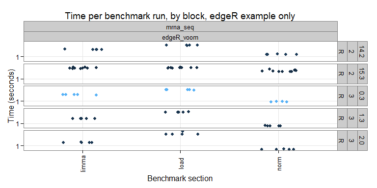
On the x-axis we have the individual sections, and the y-axis the timing (elapsed time in seconds). It is nice to see that the timings are pretty consistent within a given R version and section. I wonder if more variation would be seen benchmarks using parallel computing?
The full results for this test run can be seen here:
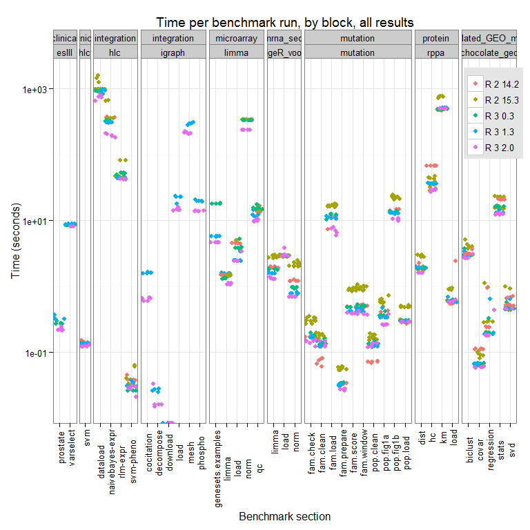
We can see differences across the R versions and the trend appears to be that newer = faster, though there are some cases where R-2.14.2 (the oldest version we test here), outperforms all other versions tested. We are looking into why this might be.
Perhaps a better way to view this is to look at the total time for each benchmark (summing all the microbenchmarks), and scale to the lowest R version tested has an average value of 100:
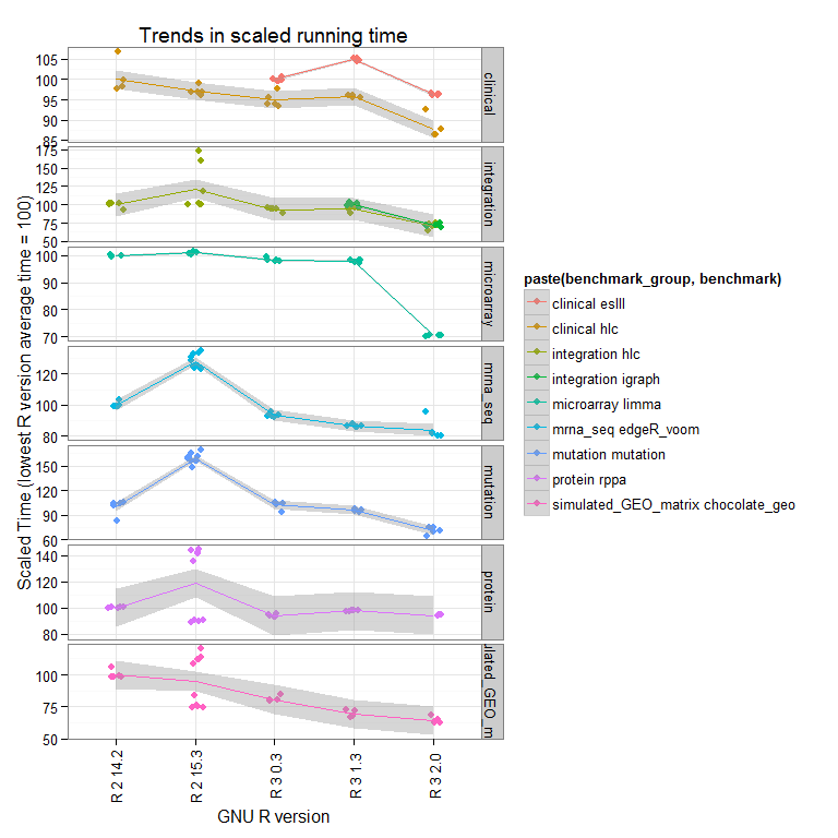
Now we see that the overall trend is that newer versions perform better overall, and that R-2.15.3 does some strange things (we are running further tests to see if this is reproducible).
Some quick stats on those trends, looking for significant differences in time across the microbenchmarks when comparing the different versions of GNU R tested (using both a parametric and non-parametric test):
res_np <- lapply(
  split(res, paste(res$benchmark_group,res$benchmark, res$block)),
  function(grp){
    param <- lm(data=grp, value~factor(paste(lang_major, lang_minor)))
    param <- as.data.frame(anova(param))
    test <- kruskal.test(data=grp, value~factor(paste(lang_major, lang_minor)))
    data.frame(
          # non parametric
          df=test$parameter, chisq=test$statistic,
          kruskal.logp=log10(test$p.value),
          # parametric
          f=param[1,"F value"], anova.logp=log10(param[1,"Pr(>F)"])
               )
    }
  )
res_np <- lapply(names(res_np), function(x){
  rownames(res_np[[x]]) <- x
  return(res_np[[x]])}
  )
Let's have a look at the top results, sorted by Kruskal-Wallis:
| df | chisq | kruskal.logp | f | anova.logp | |
|---|---|---|---|---|---|
| mrna_seq edgeR_voom norm | 4 | 27.43 | -4.79 | 265.20 | -19.35 |
| mutation mutation fam.score | 4 | 27.43 | -4.79 | 557.42 | -23.31 |
| mrna_seq edgeR_voom limma | 4 | 27.43 | -4.79 | 325.74 | -20.44 |
| mutation mutation fam.prepare | 4 | 26.74 | -4.65 | 430.87 | -21.93 |
| mutation mutation pop.fig1b | 4 | 26.58 | -4.62 | 328.81 | -20.49 |
and the bottom:
| df | chisq | kruskal.logp | f | anova.logp | |
|---|---|---|---|---|---|
| mrna_seq edgeR_voom load | 4 | 1.44 | -0.08 | 1.25 | -0.50 |
| simulated_GEO_matrix chocolate_geo svd | 4 | 3.74 | -0.35 | 1.53 | -0.65 |
| integration igraph decompose | 1 | 2.53 | -0.95 | 3.99 | -1.09 |
| protein rppa km | 4 | 7.98 | -1.03 | 3.67 | -1.74 |
| simulated_GEO_matrix chocolate_geo regression | 4 | 9.01 | -1.21 | 0.69 | -0.22 |
Interesting to see that the biggest performance changes are found in iterative tasks and not in data loading or well-established statistics, for example in the "mrna_seq / edgeR" benchmark, we only see a significant difference for computing on the data, not for loading. But considering that the data loading represents most of the time, this represents only a small gain overall. This also illustrates the importance of having ecologically valid benchmarks, because though updating R does bring speedups, for the informatician at the bench there is limited benefit as the speedups are not global.
Conclusions
To the best of our knowledge, GenBench currently provides the most comprehensive suite of real-world benchmarks for genomics. Using these benchmarks, we have demonstrated that performance improves as new versions of R are released. However, speedups are not global as only iterative tasks show significant improvements.
Going forward, we will work on extending these benchmarks as much as possible and to include the usage of (more) Bioconductor packages. The ultimate goal is to compare the performance of Renjin versus GNU R as we make improvements to Renjin's internals.
Feedback, bugs, pull requests, comments, are all more than welcome! We include a "TEMPLATE" benchmark to make it easy for people to add their own ideas.
The Benchmarks
We conclude with some background on the data and the code behind the benchmarks.
The Data
All data is publicly available, sourced from various places (for further information please see the individual README files accompanying each benchmark in the GitHub repository):
(a) Gene Expression Data - 3' Microarray - Ramsey and Fontes, 2013 - dataset - data - full article
- mRNAseq
- Data sourced from ReCount
- Specifically, the "gilad" study, PMID: 20009012
- Data sourced from ReCount
(b) Protein Expression Data - RPPA platform - Data was sourced from Hoadley et al, using the TCGA portal - Mass Spectrometry is not yet implemented
(c) Genetics Data - Population studies were simulated using data from the AML paper authored by the TCGA consortium - Pedigree studies were simulated using data obtained from the nice people at Genomes Unzipped, who make their own genomic data publicly available
(d) Simulated matrices (to allow for testing scale, as in orginal GenBase project)
(e) Clinical data and Data Integration - Data sourced from package ncvreg, further references below:
- heart dataset
- Hastie, T., Tibshirani, R., and Friedman, J. (2001). The Elements of Statistical Learning. Springer.
- Rousseauw, J., et al. (1983). Coronary risk factor screening in three rural communities. South African Medical Journal, 64, 430-436.
- prostate dataset
- Hastie, T., Tibshirani, R., and Friedman, J. (2001). The Elements of Statistical Learning. Springer.
- Stamey, T., et al. (1989). Prostate specific antigen in the diagnosis and treatment of adenocarcinoma of the prostate. II. Radical prostatectomy treated patients. Journal of Urology, 16: 1076-1083.
- lung dataset
- package survival
- Kalbfleisch D and Prentice RL (1980), The Statistical Analysis of Failure Time Data. Wiley, New York.
-
gene RIFs provided interaction data to be used for graphical modelling with igraph
- We also reproduce aspects of integrative analysis carried out in the Human Liver Cohort project:
- Hastie, T., Tibshirani, R., and Friedman, J. (2001). The Elements of Statistical Learning. Springer.
The Code
(a) Gene Expression Data - 3' Microarray Methods typical for microarrays including RMA and MAS150 normalisation, differential expression with limma, and some gene-set tests.
- mRNAseq Methods typical for mRNAseq expression analyses, including the Voom/edgeR/limma approach (The "DEseq" approach is to come).
(b) Protein Expression Data Focussing on classification, RPPA data from Hoadley et al was used a range of unpsupervised clustering methods including hierarchical, kmeans, random forrest, bayesian
(c) Genetics Data This section is still quite under-developed, focussing on summarisation of allele frequencies, and some sliding window methods. Implementation of "proper" genetics analysis methods is a burning priority!
(d) Simulated data Focus on the linear algebra and stats operations below:
- Linear Regression: build regression model to predict drug response from expression data
-
Covariance: determine which pairs of genes have expression values that are correlated
-
SVD: reduce the dimensionality of the problem to the top 50 components
-
Biclustering: simultaneously cluster rows and columns in the expression matrix to find related genes
-
Statistics: determine if certain sets of genes are highly expressed compared to the entire set of genes
-
(e) Clinical data and Data Integration Alongside some graphical methods using iGraph, we focus on machine learning approaches including clustering, and prediction using naive Bayes and robust linear model approaches
Read more at Renjin's blog or subscribe to the blog's RSS feed.